 's
Scientific Python Tools
's
Scientific Python Tools
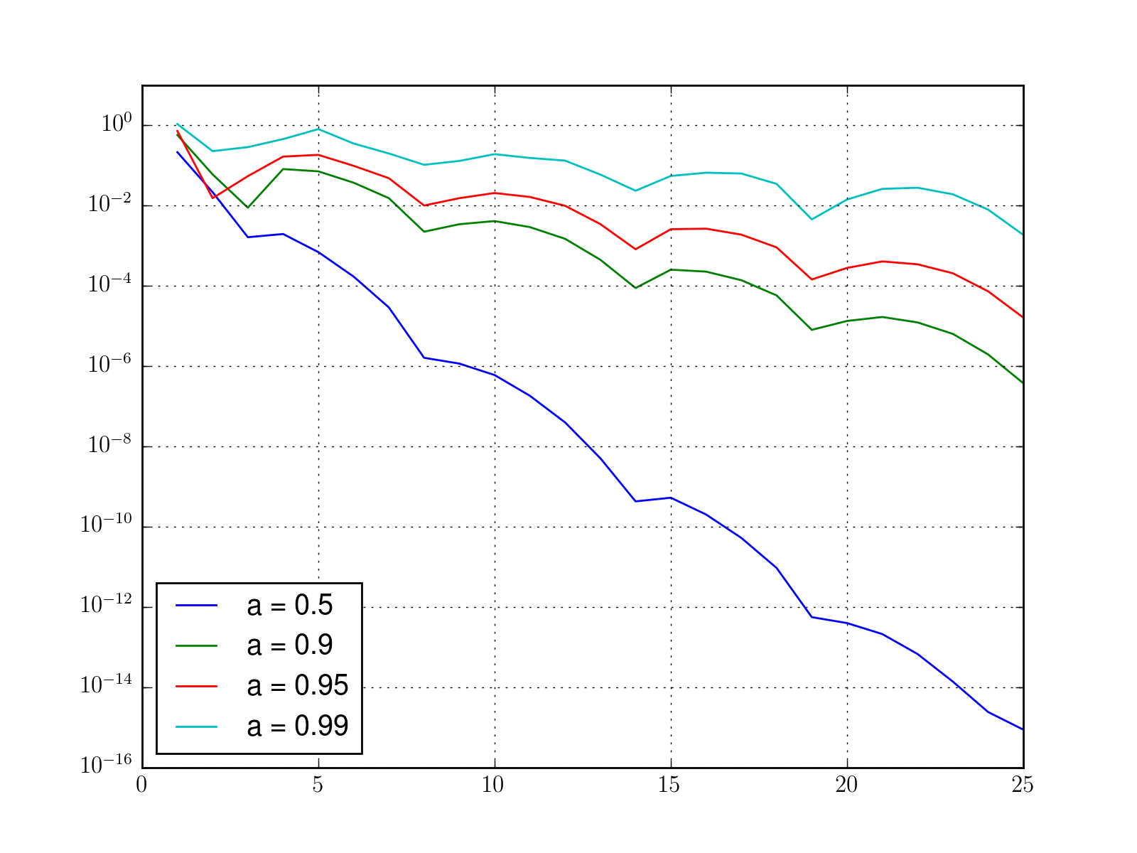
Here we put a few complete examples that should be relevant for the numerics lectures.
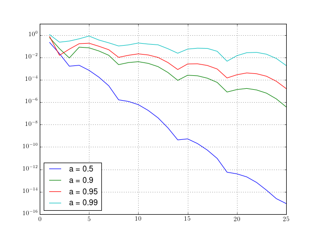
Define  .
.
We want to plot the error made by using the trapezoidal rule when
approximating  and
and  .
.
As exact value we take the value of the integral as produced by the function quad from the sub-package integrate of scipy. This function is just a wrapper to the Fortran library QUADPACK. Please, use IPython facility to consult the documentation of it.
The aim of the plots is to put in evidence the exponential convergence
of the trapezoidal rule when the smoothness of the function extends
above its periodical domain. The plots should be done for several
possible parameters  .
.
from numpy import *
from matplotlib.pyplot import *
from scipy import integrate

def trapr(func, a, b, N):
    x = linspace(a,b, N+1)
    h = x[1] - x[0]
    res = sum(func(x[1:-1])) + 0.5*(func(x[0])+func(x[-1]))
    res = res * h
    return res

# number of quadrature points used
N = 25

# integration limits
left = 0.0
right = 1.0

# alocate space for results
res = zeros(N)

lista = [0.5, 0.9, 0.95, 0.99]

for a in lista:
    myf = lambda x: 1./sqrt(1.0 - a*sin(2*pi*x-1))
    for n in xrange(N):
        res[n] = trapr(myf, left, right, n+1)

    exact, aerr = integrate.quad(myf, left, right)

    print("a: "+str(a))
    print("quad: "+str(exact))
    print("aerr: "+str(aerr))

    err = abs(res-exact)
    semilogy(arange(1,N+1), err, label="a = "+str(a))

grid(True)
legend(loc="lower left")
show()
(Source code, png, hires.png, pdf)
At lines 1-3 we import the libraries we are using. At lines 5-10 we define our quadrature rule function. Note that there are several possibilities to prepare the array of sampling points. The integrand is evaluated once at all points (vectorial) and the function sum of numpy is used in order to add the necessary values in most efficient way possible.
After preparing the data, we run the loop over the interesting values of the parameter a.
At line 25 we define the function to be integrated as a lambda function. Note that if we define it as a function of two parameters, we’d have difficulties in the later call of the trapr function.
We would like to have a program that computes both integrals and makes both plots at one. Here’s a possibility:
from numpy import *
from matplotlib.pyplot import *
from scipy import integrate

def trapr(func, a, b, N):
    """
    Compute the integral from a to b of func via trap. rule with N points
    """
    x = linspace(a,b, N+1)
    h = x[1] - x[0]
    res = sum(func(x[1:-1])) + 0.5*(func(x[0])+func(x[-1]))
    res = res * h
    return res

def ploterr(left, right, N, lista, pf):
    # allocate space for results
    res = zeros(N)

    for a in lista:
        myf = lambda x: 1.0/sqrt(1.0- a*sin(2*pi*x-1))

        for n in xrange(N):
            res[n] = trapr(myf, left, right, n+1)

        exact, aerr = integrate.quad(myf, left, right)

        print("a: "+str(a))
        print("quad: "+str(exact))
        print("aerr: "+str(aerr))

        err = abs(res-exact)
        pf(arange(1,N+1), err, label="a = "+str(a))

    grid(True)
    legend(loc="lower left")
    savefig("err"+str(right)+".png")
    close()


# not really necessary here, but you see how to do modules and test them
if __name__ == "__main__":
    lista = [0.5, 0.9, 0.95, 0.99]

    ploterr(0., 1., 25, lista, pf=semilogy)
    ploterr(0., 0.5, 100, lista, pf=loglog)
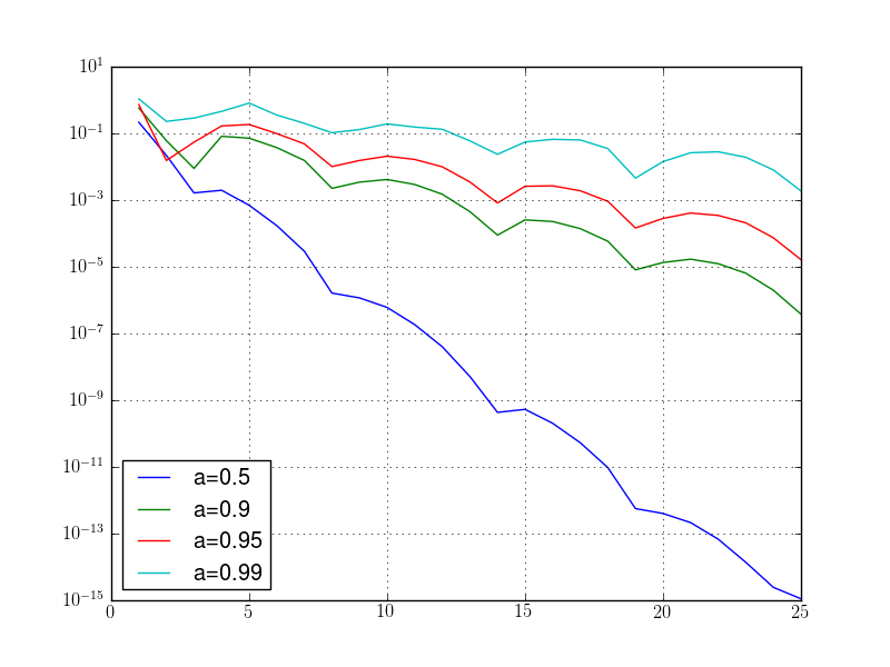
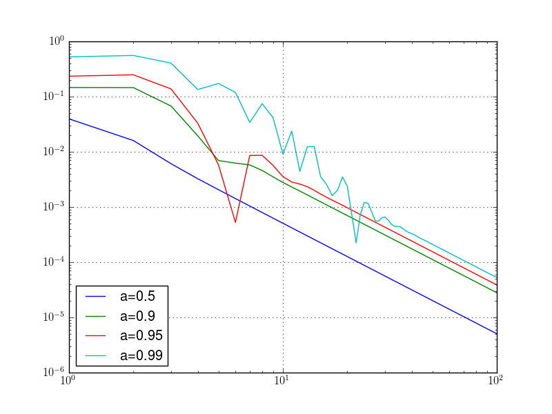
In last code, we incorporated the loop in a function that gets the integration range, the list of wished parameters and the preferred plot function (semilogy is better for the identification of the exponential convergence). The type of the file is decided by the extension of the name of the file. Note also the string concatenation used in the construction of the file name.
Finally, we would like to rewrite the code such that we avoid the trick based on inlining and locality of the variable a. We have now the occasion to see a very powerful trait of python: class function.
from numpy import *
from matplotlib.pyplot import *
from scipy import integrate

def trapr(func, a, b, N):
    """
    Compute the integral from a to b of func via trap. rule with N points
    """
    x = linspace(a,b, N+1)
    h = x[1] - x[0]
    y = func(x)
    res = sum(y[1:-1]) + 0.5*(y[0]+y[-1])
    res = res * h
    return res

class Myf(object):
    """
    models a parametric function suited for evidencing
    exponential convergence of trap. rule
    """
    def __init__(self, ina):
        self.a = ina

    def __str__(self):
        return str(self.a)

    def __call__(self, x):
        return 1.0/sqrt(1.0- self.a*sin(2*pi*x-1))

def ploterr(f, left, right, N, lista, pf):
    # allocate space for results
    res = zeros(N)

    for a in lista:
        f.a = a
        print(f)

        for n in xrange(N):
            res[n] = trapr(f, left, right, n+1)

        exact, aerr = integrate.quad(f, left, right)

        print("a: "+str(a))
        print("quad: "+str(exact))
        print("aerr: "+str(aerr))

        err = abs(res-exact)
        pf(arange(1,N+1), err, label="a="+str(a))

    grid(True)
    legend(loc="lower left")
    savefig("err"+str(right)+".png")
    close()


# not really necessary here, but you see how to do modules and test them
if __name__ == "__main__":
    lista = [0.5, 0.9, 0.95, 0.99]

    # initialize the function
    myf = Myf(0.5)

    ploterr(myf, 0., 1., 25, lista, pf=semilogy)
    ploterr(myf, 0., 0.5, 100, lista, pf=loglog)
The class Myf creates a callable objects. On line 61 we create one such object that models our parameter function, having the parameter set by the first element of the list of interesting parameters. During the loop at line 34, we modify the parameter of the object, which we use as a function to be integrated by our quadrature routines at lines 39 and 41.
This is a very simple example, but imagine the power at your hands given by the class function when you have to optimize a very complicated function (e.g. given only implicitly as the result of complicated algorithms) depending on several parameters.
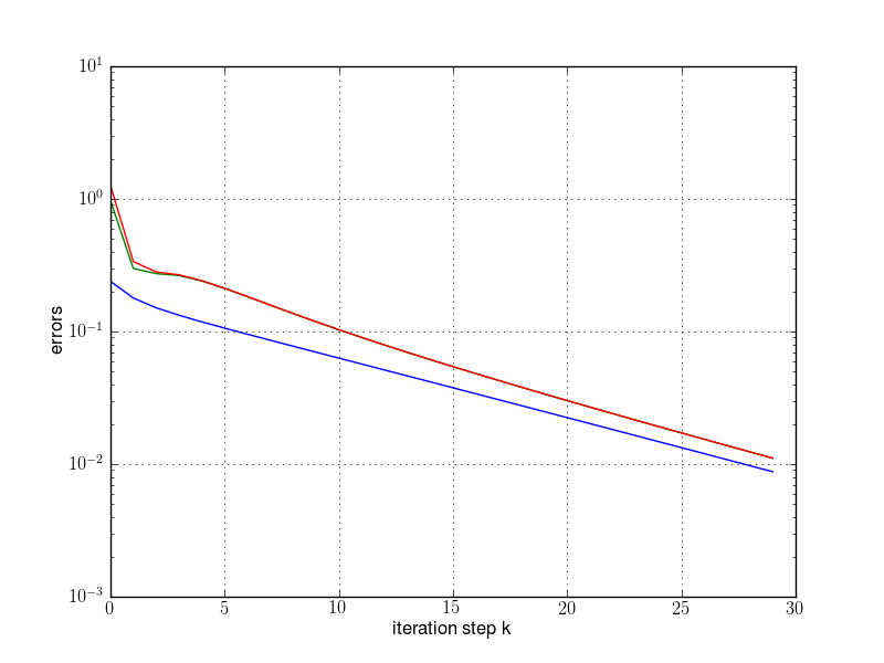
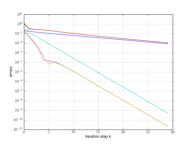
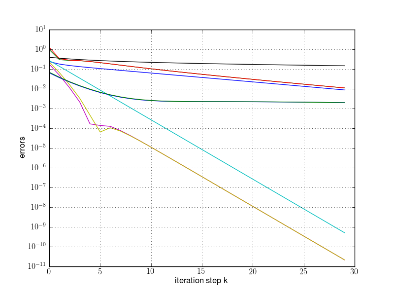
"""
Calculates eigenvalues through direct power method

Originaly, there were the input parameters d and maxit,
but in the skript, d = [1:10] and maxit = 30 are used.
"""

import numpy as np
from matplotlib import pyplot as plt

def pm(A, z, sgn, ev, ew, maxit=30):
    """Performs 'maxit' iterations of the power method
    for the matrix 'A' and the initial vector 'z'
    and computes the error for the largest eigenvalue 'ew'
    having the sign 'sgn' and the corresponding eigenvector 'ev'
    """
    res = np.zeros((maxit,5))
    s = 1;
    for k in xrange(maxit):
        w = np.dot(A,z)
        no = np.linalg.norm(w)
        rq = np.real(np.vdot(w,z))
        z = w/no
        err_aew = abs(no-abs(ew))
        err_ew = abs(sgn*rq-ew)
        err_ev = np.linalg.norm(s*z-ev)
        res[k] = np.array([k, no, err_ev, err_aew, err_ew])
        s = s*sgn
    return res

def runpm(d, fname):
    """Performs the analysis of the power iteration starting from
    the array of eigenvalues d; the picture with the results goes
    to the file indicate by fname
    """
    n = len(d) # size of the matrix
    S = np.triu(np.diag(np.r_[n:0:-1]) + np.ones((n,n)))
    A = np.dot(S, np.dot(np.diag(d), np.linalg.inv(S)))

    # need exact ew and ew for error calculation
    w, V = np.linalg.eig(A)
    t = np.where(w == abs(w).max())
    k = t[0]
    if len(k) > 1:
        raise ValueError("Error: no single larges EV")
    ev = V[:,k[0]]
    ev /= np.linalg.norm(ev)
    ew = w[k[0]]

    sgn = 1
    if ew < 0:
        sgn = -1

    print("ew:")
    print(ew)
    print("sgn:")
    print(sgn)
    print("ev =")
    print(ev)

    z = np.random.rand(n)
    z /= np.linalg.norm(z)
    res = pm(A,z,sgn,ev,ew)

    plt.semilogy(res[:,0], res[:,2])
    plt.semilogy(res[:,0], res[:,3])
    plt.semilogy(res[:,0], res[:,4])
    plt.grid(True)
    plt.xlabel("iteration step k")
    plt.ylabel("errors")
    plt.savefig(fname)
    plt.show()


if __name__=="__main__":
    # size of the matrix
    n = 10

    d = 1.0 + np.arange(n) # eigenvalues
    print("d:")
    print(d)
    print("d[-2]/d[-1]:")
    print(d[-2]/d[-1])
    runpm(d, "pm1.png")

    d = np.ones(n)
    d[-1] = 2.0 # eigenvalues
    print("d:")
    print(d)
    print("d[-2]/d[-1]:")
    print(d[-2]/d[-1])
    runpm(d, "pm2.png")

    d = 1.0 - 0.5**np.linspace(1,5,9) # eigenvalues
    print("d:")
    print(d)
    print("d[-2]/d[-1]:")
    print(d[-2]/d[-1])
    runpm(d, "pm3.png")
Serial Monte-Carlo integration via IPython. Serial code:
"""
 Computes integral
 I0(1) = (1/pi) int(z=0..pi)  exp(-cos(z)) dz by raw MC.
 Abramowitz and Stegun give I0(1) = 1.266066
"""

import numpy as np
import time

t1 = time.time()

# number of times we run our MC inetgration
M = 100
asval = 1.266065878

ex = np.zeros(M)

print("A and S tables:  I0(1) = "+str(asval))
print("sample       variance        MC I0 val")
print("------       --------        ---------")

# how many experiments
k = 5
N = 10**np.arange(1,k+1)
v = []
e = []

for n in N:
    for m in xrange(M):
        x = np.random.rand(n)
        x = np.exp(np.cos(-np.pi*x))
        ex[m] = sum(x)/n

    ev = sum(ex)/M
    vex = np.dot(ex,ex)/M
    vex -=  ev**2
    v += [vex]
    e += [ev]
    print((n, vex, ev))

t2 = time.time()
t = t2 - t1

print("Serial calculation completed, time = "+str(t)+" s")
Output:
A and S tables:  I0(1) = 1.266065878
sample       variance        MC I0 val
------       --------        ---------
(10, 0.069908462650839942, 1.2525905567351583)
(100, 0.0055876950073416864, 1.2709643005937217)
(1000, 0.0006511488699125767, 1.262876852977836)
(10000, 5.7940507106613026e-05, 1.2664260011112918)
(100000, 6.7123607208063873e-06, 1.265782558306026)
Serial calculation completed, time = 5.22518420219 s
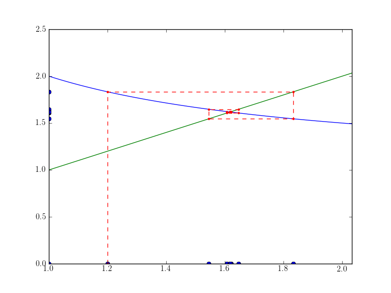
A nice plot showing the fixed-point iteration in action finding the golden ration.
from numpy import *
from matplotlib.pyplot import *

phi = lambda x: (1.0 + 1.0/(1.0*x))
#phi = lambda x: sqrt(x+1.0)

x0 = 1.2

x = [x0]
y = [0]

for i in xrange(10):
    x1 = phi(x0)

    x.append(x0)
    y.append(x1)

    x.append(x1)
    y.append(x1)

    x0 = x1

x = array(x)
y = array(y)

xmin = x.min() - 0.2
xmax = x.max() + 0.2

t = linspace(xmin, xmax, 50)

figure()
plot([xmin, xmax], [xmin, xmax], "g")
plot(t, phi(t), "b")

plot(x, zeros_like(x), "bo")
plot(xmin*ones_like(y), y, "bo")

plot(x, y, "r--")
plot(x, y, "r.")

xlim(xmin, xmax)
savefig("spiral1.png")

print(x)
print(y)