 's
Scientific Python Tools
's
Scientific Python Tools
The most important and central python package for doing scientific computing is NumPy. This package provides convenient and fast arbitrary-dimensional array manipulation routines. The home of NumPy as well as some other scientific packages is:
We will give a very short introduction to NumPy now.
The main python object is a N-dimensional array data structure. In the following sections we show different core aspects of this array object.
The NumPy arrays have three fundamental properties.
- shape: The shape attribute of any arrys describes its size
along all of its dimensions
ndim: The number of dimensions (often also called directions or axes)
dtype: The data type of the array elements.
Lets look at some examples to get a feeling for these concepts. At the very beginning we make sure to import (load) the numpy python module (package):
In [1]: from numpy import * # Import all (top-level) functions from numpy
We can create arrays from (nested) python lists or tuples:
In [2]: A = array([1,2,3,4,5])

In [3]: A
Out[3]: array([1, 2, 3, 4, 5])

In [4]: type(A)
Out[4]: numpy.ndarray
This is a simple vector of 5 elements. The type of the array itself is numpy.ndarray. The array is one-dimensional as expected:
In [5]: A.ndim
Out[5]: 1
and has the following shape (shapes are always return as python tuples)
In [6]: A.shape
Out[6]: (5,)
The data type of the elements of A is:
In [7]: A.dtype
Out[7]: dtype('int64')
But most of the time we don’t need to bother us with types. Let’s create a simple matrix:
In [10]: M = array([[1,2,3],[4,5,6]])

In [11]: M
Out[11]:
array([[1, 2, 3],
       [4, 5, 6]])
We should think of matrices simply as two-dimensional arrays:
In [12]: M.ndim
Out[12]: 2
This one having two rows and three columns:
In [13]: M.shape
Out[13]: (2, 3)
We could define higher-dimensional arrays too but will do this rarely.
The full specification of the ndarray object can be read at:
There are several other methods to construct arrays beside the initialization by nested lists. Remember that the list can also be a list comprehension:
In [23]: S = array([i**2 for i in xrange(10)])

In [24]: S
Out[24]: array([ 0,  1,  4,  9, 16, 25, 36, 49, 64, 81])
We will learn a much better way later to achieve the same. It is possible to use lambda functions together with nested list comprehensions for advanced matrix constructions. In the following we build a so-called Toeplitz matrix:
In [25]: arc = lambda r,c: r-c

In [26]: T = array([[arc(r,c) for c in xrange(4)] for r in xrange(5)])

In [27]: T
Out[27]:
array([[ 0, -1, -2, -3],
       [ 1,  0, -1, -2],
       [ 2,  1,  0, -1],
       [ 3,  2,  1,  0],
       [ 4,  3,  2,  1]])
Often we want to initialize arrays for later use. For example we can create arrays of zeros or ones by these two functions of same name:
In [14]: Z = zeros((12,))

In [15]: Z
Out[15]: array([ 0.,  0.,  0.,  0.,  0.,  0.,  0.,  0.,  0.,  0.,  0.,  0.])

In [16]: O = ones((3,3))

In [17]: O
Out[17]:
array([[ 1.,  1.,  1.],
       [ 1.,  1.,  1.],
       [ 1.,  1.,  1.]])
Identity matrices can be made with eye:
In [34]: I = eye(3)

In [35]: I
Out[35]:
array([[ 1.,  0.,  0.],
       [ 0.,  1.,  0.],
       [ 0.,  0.,  1.]])
If we need N equally spaced points between two endpoints a and b we can call linspace(a, b, N) like:
In [38]: points = linspace(0, 10, 15)

In [39]: points.shape
Out[39]: (15,)

In [40]: points
Out[40]:
array([  0.        ,   0.71428571,   1.42857143,   2.14285714,
         2.85714286,   3.57142857,   4.28571429,   5.        ,
         5.71428571,   6.42857143,   7.14285714,   7.85714286,
         8.57142857,   9.28571429,  10.        ])
If we need only some integer ranges, we can either convert the result of Python’s range or directly call NumPy’s arange (remember that the last point is always excluded in ranges but included in the result of linspace):
In [53]: array(range(5,13))
Out[53]: array([ 5,  6,  7,  8,  9, 10, 11, 12])

In [54]: arange(5,13)
Out[54]: array([ 5,  6,  7,  8,  9, 10, 11, 12])
For computing a two-dimensional grid of points there is the meshgrid command. We show only a small example here:
In [43]: x = linspace(0, 3, 4)

In [44]: x
Out[44]: array([ 0.,  1.,  2.,  3.])

In [45]: y = linspace(0, 2, 3)

In [46]: y
Out[46]: array([ 0.,  1.,  2.])

In [47]: X,Y = meshgrid(x,y)

In [48]: X
Out[48]:
array([[ 0.,  1.,  2.,  3.],
       [ 0.,  1.,  2.,  3.],
       [ 0.,  1.,  2.,  3.]])

In [49]: Y
Out[49]:
array([[ 0.,  0.,  0.,  0.],
       [ 1.,  1.,  1.,  1.],
       [ 2.,  2.,  2.,  2.]])
Meshgrids are commonly used for plotting in three dimensions.
Sometimes we already have an array and want to create another one with same shape. For this we have the functions zeros_like and ones_like at hand:
In [50]: zeros_like(T)
Out[50]:
array([[0, 0, 0, 0],
       [0, 0, 0, 0],
       [0, 0, 0, 0],
       [0, 0, 0, 0],
       [0, 0, 0, 0]])

In [52]: ones_like(A)
Out[52]: array([1, 1, 1, 1, 1])
Finally, from time to time we need random numbers. There are powerful methods for filling arrays with random numbers [1]. The most simple call looks like:
In [58]: random.random((3,5))
Out[58]:
array([[ 0.79921796,  0.01877047,  0.56102347,  0.57946688,  0.37414866],
       [ 0.84593219,  0.44403091,  0.89057679,  0.11296198,  0.72045779],
       [ 0.40033809,  0.81665445,  0.07307056,  0.24462193,  0.8721881 ]])
and gives us values according to the continuous uniform distribution on  .
.
More on array creation can be found in the NumPy reference:
Indexing some single value or even a whole set of values from a given array is the next important operation we need to learn about.
Indexing for retrieving single elements works as usual in python and indexing by negative numbers starts counting from the end:
In [63]: l = arange(9)

In [64]: l
Out[64]: array([0, 1, 2, 3, 4, 5, 6, 7, 8])

In [65]: l[3]
Out[65]: 3

In [66]: l[-2]
Out[66]: 7
We run into IndexError exceptions if we try to access elements not available:
In [69]: l[9]
---------------------------------------------------------------------------
IndexError                                Traceback (most recent call last)
<ipython-input-69-622e6bac6342> in <module>()
----> 1 l[9]

IndexError: index out of bounds

In [74]: l[-10]
---------------------------------------------------------------------------
IndexError                                Traceback (most recent call last)
<ipython-input-74-3f63644bd4e3> in <module>()
----> 1 l[-10]

IndexError: index out of bounds
In general we have to index an array A with as many indices as there are dimensions (There are some more or less esoteric exceptions).
In [75]: A = eye(4)

In [76]: A
Out[76]:
array([[ 1.,  0.,  0.,  0.],
       [ 0.,  1.,  0.,  0.],
       [ 0.,  0.,  1.,  0.],
       [ 0.,  0.,  0.,  1.]])

In [77]: A[0,0]
Out[77]: 1.0

In [78]: A[0,3]
Out[78]: 0.0

In [80]: A[1,1,1]
---------------------------------------------------------------------------
IndexError                                Traceback (most recent call last)
<ipython-input-80-97042a7c163c> in <module>()
----> 1 A[1,1,1]

IndexError: invalid index
In principle we can also index A by just one value and get:
In [79]: A[1]
Out[79]: array([ 0.,  1.,  0.,  0.])
we will learn later how to interpret this result. In any case you should be very careful with such things.
The term slicing is used for extracting whole rows, columns or other rectangular (hypercubic) subregions from an arbitrary dimensional array. One can easily select the colored regions from the following images.
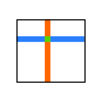
We can extract (slice out) single rows or columns by indexing with colons;
In [130]: A = array([[1,2,3,4],[5,6,7,8],[9,10,11,12]])

In [131]: A
Out[131]:
array([[ 1,  2,  3,  4],
       [ 5,  6,  7,  8],
       [ 9, 10, 11, 12]])

In [132]: r1 = A[1,:]   # Get the second row (indexing starts at 0)

In [133]: r1
Out[133]: array([5, 6, 7, 8])

In [134]: r1.shape
Out[134]: (4,)

In [135]: c2 = A[:,2]   # Get the third column (indexing starts at 0)

In [136]: c2
Out[136]: array([ 3,  7, 11])

In [137]: c2.shape
Out[137]: (3,)
Now we can also understand what A[1] does:
In [158]: A[1]
Out[158]: array([5, 6, 7, 8])
If we provide too less indices, then NumPy appends as many : as necessary to the end of the given index (tuple).
Its possible to select more that one row or column at once.
The syntax stays the same:
In [142]: A[:,0:3]   # The first three columns
Out[142]:
array([[ 1,  2,  3],
       [ 5,  6,  7],
       [ 9, 10, 11]])

In [144]: A[1:3,:]   # The second two rows
Out[144]:
array([[ 5,  6,  7,  8],
       [ 9, 10, 11, 12]])

In [146]: A[1:3,1:3]   # A submatrix slice
Out[146]:
array([[ 6,  7],
       [10, 11]])
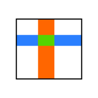
What if we want to select a non-contiguous block, like shown in the next image.
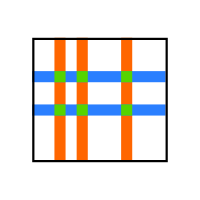
Select all orange columns? Select all blue rows? Or even all green elements? This is also possible, we just have to use tuple notation:
In [152]: A[:, (0,2,3)]
Out[152]:
array([[ 1,  3,  4],
       [ 5,  7,  8],
       [ 9, 11, 12]])

In [153]: A[(0,1),:]
Out[153]:
array([[1, 2, 3, 4],
       [5, 6, 7, 8]])
The major caveat here is the following:
In [154]: A[(0,1),(0,3)]   # What? Why did we not get 4 elements?
Out[154]: array([1, 8])

In [155]: A[(0,1),(0,2,3)]
---------------------------------------------------------------------------
ValueError                                Traceback (most recent call last)
<ipython-input-155-3c3d973d8ee2> in <module>()
----> 1 A[(0,1),(0,2,3)]

ValueError: shape mismatch: objects cannot be broadcast to a single shape
It is even possible to use arrays to index other arrays like in the following example:
In [180]: i = array([0,2])

In [181]: A[:,i]
Out[181]:
array([[ 1,  3],
       [ 5,  7],
       [ 9, 11]])

In [182]: A[i,:]
Out[182]:
array([[ 1,  2,  3,  4],
       [ 9, 10, 11, 12]])
This is the key to solve our failed index example from above. We can indeed select the 6 non-contiguous single elements and get the result packet into a two-dimensional array:
In [160]: u=array([[0,1]])

In [161]: u
Out[161]: array([[0, 1]])

In [162]: v=array([[0],[2],[3]])

In [163]: A[u,v]
Out[163]:
array([[1, 5],
       [3, 7],
       [4, 8]])
As a last example lets look at so called boolean indexing where we select all elements having some common property:
In [188]: a
Out[188]: array([[0, 1, 2, 3, 4]])

In [190]: A = a*transpose(a)

In [191]: A
Out[191]:
array([[ 0,  0,  0,  0,  0],
       [ 0,  1,  2,  3,  4],
       [ 0,  2,  4,  6,  8],
       [ 0,  3,  6,  9, 12],
       [ 0,  4,  8, 12, 16]])

In [192]: A[A>=6]   # Select all elements from A that are larger than 6
Out[192]: array([ 6,  8,  6,  9, 12,  8, 12, 16])
A special case of indexing is iteration where we iterate in a loop over all elements of an array (in row-wise fashion) like over the elements of a simple python list. For multi-dimensional array we have to flatten it first.
In [198]: [i**2 for i in A.flatten()]
Out[198]:
[0,
 0,
 0,
 0,
 0,
 0,
 1,
 4,
 9,
 16,
 0,
 4,
 16,
 36,
 64,
 0,
 9,
 36,
 81,
 144,
 0,
 16,
 64,
 144,
 256]
If you still want to learn more about the NumPy indexing and slicing features, there is a whole section in the reference:
We can stack together arrays (with matching shapes of course) along the first (rows) or second (columns) axes:
In [13]: A = arange(4)

In [14]: B = vstack([A,A,A])

In [15]: B
Out[15]:
array([[0, 1, 2, 3],
       [0, 1, 2, 3],
       [0, 1, 2, 3]])

In [8]: C = array([[1,2],[3,4]])

In [9]: C
Out[9]:
array([[1, 2],
       [3, 4]])

In [10]: D = hstack([C,C])

In [11]: D
Out[11]:
array([[1, 2, 1, 2],
       [3, 4, 3, 4]])
Another useful operation is reshaping of arrays. The condition for this operation is that both shapes will result in the same number of elements.
In [17]: B.reshape((6,2))
Out[17]:
array([[0, 1],
       [2, 3],
       [0, 1],
       [2, 3],
       [0, 1],
       [2, 3]])
Note that the elements get filled in in row-wise order or more general the elements are taken along the last axes first. In the extreme case we can make the array with a singular dimension:
In [23]: B.reshape((12,1))
Out[23]:
array([[0],
       [1],
       [2],
       [3],
       [0],
       [1],
       [2],
       [3],
       [0],
       [1],
       [2],
       [3]])

In [24]: E = B.reshape((12,1))

In [25]: E.shape
Out[25]: (12, 1)

In [26]: E.ndim
Out[26]: 2
Note that E is still two-dimensional but with shape 1 along the second axis (this is called a singular dimension). This can be inconvenient in some cases (for example for plotting as we will see later). The solution to this is called squeeze and removes all singular dimensions of an array:
In [28]: F = squeeze(E)

In [29]: F
Out[29]: array([0, 1, 2, 3, 0, 1, 2, 3, 0, 1, 2, 3])

In [30]: F.ndim
Out[30]: 1

In [31]: F.shape
Out[31]: (12,)

In [53]: oneelem = array([[5]])   # A matrix with one single element

In [54]: oneelem
Out[54]: array([[5]])

In [55]: oneelem.ndim
Out[55]: 2

In [56]: oneelem.shape
Out[56]: (1, 1)

In [57]: scalar = squeeze(oneelem)

In [58]: scalar.shape
Out[58]: ()

In [59]: scalar.ndim
Out[59]: 0
Finally there is the important transpose operation which acts as a transpose in the mathematical sense:
In [61]: B
Out[61]:
array([[0, 1, 2, 3],
       [0, 1, 2, 3],
       [0, 1, 2, 3]])

In [70]: B.shape
Out[70]: (3, 4)

In [62]: transpose(B)
Out[62]:
array([[0, 0, 0],
       [1, 1, 1],
       [2, 2, 2],
       [3, 3, 3]])

In [68]: TB = transpose(B)

In [69]: TB.shape
Out[69]: (4, 3)
It’s important to note that we can only transpose arrays of dimension larger than 1.
In [63]: A
Out[63]: array([0, 1, 2, 3])

In [65]: A.shape
Out[65]: (4,)

In [66]: TA = transpose(A)

In [71]: TA
Out[71]: array([0, 1, 2, 3])

In [67]: TA.shape
Out[67]: (4,)
An option would be to reshape A to (1,4) and then take the transpose. Because this is a very common operation there is a small helper function called atleast_2d which does the job:
In [72]: TA2 = transpose(atleast_2d(A))

In [73]: TA2
Out[73]:
array([[0],
       [1],
       [2],
       [3]])

In [74]: TA2.shape
Out[74]: (4, 1)
An overview of many more useful methods to manipulate arrays as a whole is given here:
Until now we have only worked with arrays as structured data containers. Usually we want to work with the the data inside too.
Arrays support all basic arithmetic operation out of the box:
In [113]: a = arange(4)

In [114]: a
Out[114]: array([0, 1, 2, 3])

In [115]: a+a
Out[115]: array([0, 2, 4, 6])

In [116]: a-a
Out[116]: array([0, 0, 0, 0])

In [117]: a*a
Out[117]: array([0, 1, 4, 9])

In [118]: a/a
/usr/bin/ipython:1: RuntimeWarning: divide by zero encountered in divide
  #!/usr/bin/python
Out[118]: array([0, 1, 1, 1])
Note that we got a warning for the division by zero but nevertheless obtained a valid array.
Remember the computation of squares from above? Now we know how to do this in the most simple way:
In [184]: arange(10)**2
Out[184]: array([ 0,  1,  4,  9, 16, 25, 36, 49, 64, 81])
In these examples all arrays were of matching shape. But what happens if this is not the case?
If we try to perform some operation where the shapes of the operands do not match, NumPy still tries to do some computation if possible. The method applied to resolve the issue is called broadcasting and shown in the following pictures. First a simple example, we want to multiply the array a by a scalar number:

NumPy now makes an array of the same shape of a by repeating the element as many times as necessary (gray boxes). (Of course internally no memory is wasted and this second array never constructed explicitly.)
In [121]: a = arange(1,5)

In [122]: a
Out[122]: array([1, 2, 3, 4])

In [123]: a.shape
Out[123]: (4,)

In [124]: a*2
Out[124]: array([2, 4, 6, 8])

In [125]: b = a*2

In [126]: b.shape
Out[126]: (4,)
As a second example we add a row and a column vector of different length like shown in this figure:
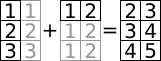
Let’s try to do this with NumPy arrays now:
In [145]: a = arange(1,4).reshape((3,1))

In [146]: a
Out[146]:
array([[1],
       [2],
       [3]])

In [147]: a.shape
Out[147]: (3, 1)

In [148]: b = array([[1,2]])

In [149]: b
Out[149]: array([[1, 2]])

In [150]: b.shape
Out[150]: (1, 2)

In [151]: c = a+b

In [152]: c
Out[152]:
array([[2, 3],
       [3, 4],
       [4, 5]])

In [153]: c.shape
Out[153]: (3, 2)
Some more explanations and examples of broadcasting can be found in the user guide:
The exact details when broadcasting is applied are stated in the reference manual:
NumPy provides a rich set of functions that operate on the elements of an array. These functions are called ufuncs (short for universal functions) and the manual says:
Each universal function takes array inputs and produces array outputs by performing the core function element-wise on the inputs.
where the core function can be for example some math function like sin:
In [81]: x = linspace(0, 2*pi, 10)

In [82]: x
Out[82]:
array([ 0.        ,  0.6981317 ,  1.3962634 ,  2.0943951 ,  2.7925268 ,
        3.4906585 ,  4.1887902 ,  4.88692191,  5.58505361,  6.28318531])

In [83]: y = sin(x)

In [84]: y
Out[84]:
array([  0.00000000e+00,   6.42787610e-01,   9.84807753e-01,
         8.66025404e-01,   3.42020143e-01,  -3.42020143e-01,
        -8.66025404e-01,  -9.84807753e-01,  -6.42787610e-01,
        -2.44929360e-16])
In the introduction we said that we don’t care about data types too much. There are some exceptions like the following example shows:
In [104]: o = -ones((2,))

In [105]: o
Out[105]: array([-1., -1.])

In [106]: sqrt(o)
Out[106]: array([ nan,  nan])

In [107]: oc = -ones((2,), dtype=complexfloating)

In [108]: oc
Out[108]: array([-1.-0.j, -1.-0.j])

In [109]: sqrt(oc)
Out[109]: array([ 0.-1.j,  0.-1.j])

In [110]: o.dtype
Out[110]: dtype('float64')

In [111]: oc.dtype
Out[111]: dtype('complex128')
A good overview of the many available ufucs can be found at:
More information about universal functions in general:
All functions we know by now operate element-wise on arrays. For linear algebra we need scalar, matrix-vector and matrix-matrix products. The function for all three is called dot and takes two operands:
In [164]: A = array([[1,2],[3,4]])

In [165]: v = array([5,6])

In [166]: dot(v, v)
Out[166]: 61

In [167]: dot(A, v)
Out[167]: array([17, 39])

In [168]: dot(A, A)
Out[168]:
array([[ 7, 10],
       [15, 22]])
In this example the vector has a shape of (2,). For one-dimensional arrays as vectors everything is fine (remember that transpose has no effect for one-dimensional arrays). We can also work with (two-dimensional) explicit column vectors:
In [172]: v = v.reshape((2,1))

In [173]: v.shape
Out[173]: (2, 1)

In [174]: A.shape
Out[174]: (2, 2)
This time the dot product failes because the shapes do not match:
In [175]: dot(v, v)
---------------------------------------------------------------------------
ValueError                                Traceback (most recent call last)
<ipython-input-175-093f352c32e0> in <module>()
----> 1 dot(v, v)

ValueError: objects are not aligned
This is a very typical error message. Whenever you see this you should go and check the shapes of your arrays again.
We have to take the transpose of the first argument, equivalent to
the mathematical formulation  :
:
In [176]: dot(transpose(v), v)
Out[176]: array([[61]])
Note that the result is still a two-dimensional array of shape (1, 1).
If this is inconvenient we could use squeeze on the result.
We can even built outer products  this way:
In [179]: dot(v, transpose(v))
Out[179]:
array([[25, 30],
       [30, 36]])
In priciple this is all very straight-forward, we just have to be careful enough with the shapes of all operands.
Footnotes
| [1] | http://docs.scipy.org/doc/numpy/reference/routines.random.html |