 's
Scientific Python Tools
's
Scientific Python Tools
The second very important python package we look at is SciPy. The SciPy documentation says:
SciPy is a collection of mathematical algorithms and convenience functions built on the Numpy extension for Python. It adds significant power to the interactive Python session by exposing the user to high-level commands and classes for the manipulation and visualization of data.
You can read a longer informal introduction at:
The home of the SciPy python package is:
In the following we will make some examples for a few selected parts of SciPy. But SciPy is a huge library and we can not make an example or point you to every useful function from it. There also is no good reason to duplicate its documentation here. If you encounter a (scientific programming) problem you should go to the library reference:
and search for the tools you need. The documentation is very good and well structured.
At the end of the last chapter we only looked at the very basics of linear algebra. In this section we show some more features.
First we have to import the linalg submodule of scipy
In [1]: from numpy import *

In [2]: from scipy.linalg import *
Let’s do a first computation:
In [5]: A = array([[1,2,3],[4,5,6],[7,8,8]])

In [6]: det(A)
Out[6]: 3.0
next we can do a LU decomposition of A:
In [11]: P, L, U = lu(A)

In [12]: L
Out[12]:
array([[ 1.        ,  0.        ,  0.        ],
       [ 0.14285714,  1.        ,  0.        ],
       [ 0.57142857,  0.5       ,  1.        ]])

In [13]: U
Out[13]:
array([[ 7.        ,  8.        ,  8.        ],
       [ 0.        ,  0.85714286,  1.85714286],
       [ 0.        ,  0.        ,  0.5       ]])

In [14]: dot(L,U)
Out[14]:
array([[ 7.,  8.,  8.],
       [ 1.,  2.,  3.],
       [ 4.,  5.,  6.]])

In [15]: dot(P,dot(L,U))
Out[15]:
array([[ 1.,  2.,  3.],
       [ 4.,  5.,  6.],
       [ 7.,  8.,  8.]])
We can find out the eigenvalues and eigenvectors of this matrix:
In [17]: EW, EV = eig(A)

In [18]: EW
Out[18]: array([ 15.55528261+0.j,  -1.41940876+0.j,  -0.13587385+0.j])

In [19]: EV
Out[19]:
array([[-0.24043423, -0.67468642,  0.51853459],
       [-0.54694322, -0.23391616, -0.78895962],
       [-0.80190056,  0.70005819,  0.32964312]])

In [20]: dot(A, EV[:,0])
Out[20]: array([ -3.74002233,  -8.50785632, -12.47378976])

In [21]: n = dot(A, EV[:,0]) - EW[0]*EV[:,0]

In [22]: n
Out[22]: array([ -3.55271368e-15+0.j,  -1.24344979e-14+0.j,  -8.88178420e-15+0.j])

In [23]: norm(n)
Out[23]: 1.5688358818848954e-14
Indeed, we found the eigenvalues and eigenvectors.
Solving systems of linear equations is not more difficult:
In [26]: v = array([[2,3,5]])

In [27]: s = solve(A, transpose(v))

In [28]: s
Out[28]:
array([[-2.33333333],
       [ 3.66666667],
       [-1.        ]])
We can check the solution:
In [29]: dot(A, s) - v
Out[29]:
array([[  4.44089210e-16,  -1.00000000e+00,  -3.00000000e+00],
       [  1.00000000e+00,   8.88178420e-16,  -2.00000000e+00],
       [  3.00000000e+00,   2.00000000e+00,   3.55271368e-15]])
Oups, broadcasting happened! We have to transpose the vector v (or squeeze the result of dot):
In [30]: dot(A, s) - transpose(v)
Out[30]:
array([[  4.44089210e-16],
       [  8.88178420e-16],
       [  3.55271368e-15]])
If you want you can read on here
to see some more examples on how to do linear algebra with SciPy.
For a complete overview of the (dense) linear algebra functionalities of SciPy please see:
SciPy has some routines for computing with sparse and potentially very large matrices. The necessary tools are in the submodule scipy.sparse.
We make one example on how to construct a large matrix:
In [1]: from scipy.sparse import *

In [2]: from scipy import rand

In [3]: A = lil_matrix((1000, 1000))

In [4]: A[0,:100] = rand(100)

In [5]: A[1,100:200] = A[0,:100]

In [6]: A.setdiag(rand(1000))

In [7]: A
Out[7]:
<1000x1000 sparse matrix of type '<type 'numpy.float64'>'
        with 1199 stored elements in LInked List format>
Next we solve a linear equation:
In [8]: from scipy.sparse.linalg import *

In [9]: A = A.tocsr()
                                                                                                                                                            In [10]: A
Out[10]:
<1000x1000 sparse matrix of type '<type 'numpy.float64'>'
        with 1199 stored elements in Compressed Sparse Row format>

In [11]: b = rand(1000)

In [12]: x = spsolve(A, b)
The two largest and smallest eigenvalues of A:
In [26]: EWs, EVs = eigs(A, 2, which="SM")

In [27]: EWs
Out[27]: array([ 0.00107174+0.j,  0.00211868+0.j])

In [28]: EWl, EVl = eigs(A, 2, which="LM")

In [29]: EWl
Out[29]: array([ 0.99854009+0.j,  0.99786107+0.j])
For further information please see the reference for sparse matrices:
and sparse linear algebra:
There are plenty of different Fourier and related transformations available.
Some function are available in the numpy.fft submodue:
others in the scipy.fftpack submodule:
It’s a bit unfortunate that some of these functions live in NumPy rather than SciPy.
SciPy has functions for univariate and multivariate as well as unconstrained and constrained optimization techniques.
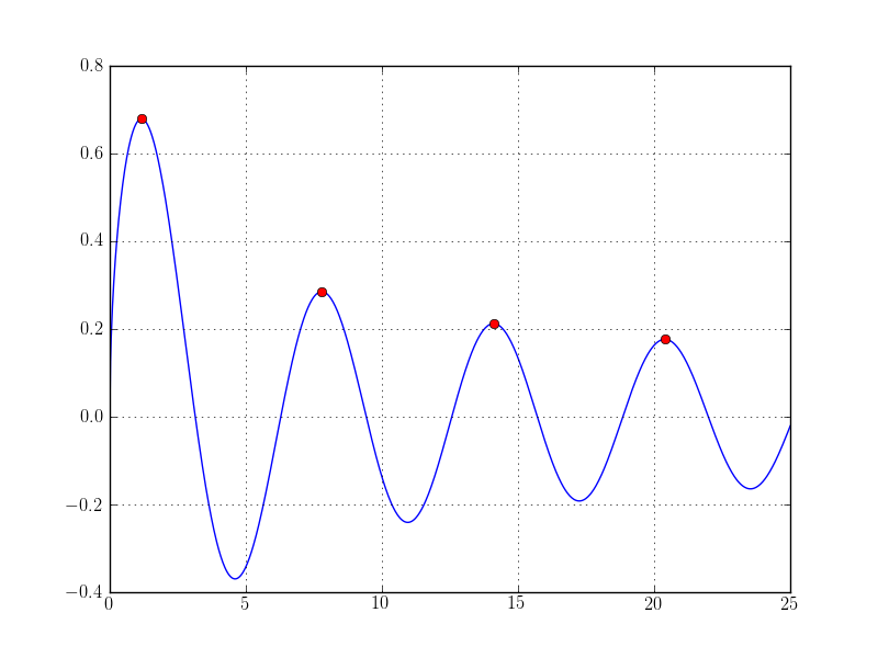
As an example we compute the first 4 maxima of the Bessel function  given an initial guess for each one and a bounded interval to search in:
In [1]: from scipy.special import jv    # Import the Bessel J_n special function

In [2]: from scipy.optimize import fminbound

In [3]: approx = [1, 6, 12, 18]

In [4]: for guess in approx:
   ...:     f = lambda x: -jv(0.5, x)
   ...:     xmax = fminbound(f, guess-4, guess+4)
   ...:     print(xmax)
   ...:
1.16556123601
7.78988391603
14.1017257582
20.3958424877
This specific Bessel function looks like:
Consult the documentation for more details on the various different routines of the scipy.optimize submodule:
- http://docs.scipy.org/doc/scipy/reference/special.html All the ususal higher special functions from mathematics and physics. Almost all of them are implemented as universal functions operating on NumPy arrays.
- http://docs.scipy.org/doc/scipy/reference/stats.html Large collection statistical functions and random distributions.
- http://docs.scipy.org/doc/scipy/reference/constants.html Physical and mathematical constants and units. The values are taken from the “CODATA Recommended Values of the Fundamental Physical Constants 2010”.
- http://docs.scipy.org/doc/scipy/reference/integrate.html Some functions for numerical integration and methods for solving ODEs.
There are many other submodules of SciPy and we have no place to introduce all. (Additionally not all are relevant for our purpose.) Anyway, if you are interested or need more information, look into the reference guide: