Symbolic calculations

Even if we want to deal with numerical computations mainly, I’d like to give a short introduction into symbolic calculation. There are several reasons why we want to include some symbolic manipulations in a numerical code. For example we want to do an error analysis and would like to be able to evaluate the known exact solution on various different grids. Or we have a closed form solution for some right hand side. Beyond the toy examples there exist also industrial strength codes that use symbolic computation in a preparation step before going into the numerics [1].

In any case, we could put the symbolic expression literally into the source code. But sometimes it would be useful if we could do a few more things with the expression beside numerical evaluation, for example we may need the first derivative. The benefit of symbolic calculation is now that we can compute this derivation without explicitly put it into the source code or falling back to numerical techniques.

In the following section I’ll show a really simple example of how to use the power of the sympy python module. This module acts as a library for symbolic calculation and is quite easy to use yet surprisingly powerful for it’s complexity.

# Use explicit namespaces to make clear from which package a function comes.
import sympy as sp
import numpy as np
import matplotlib.pyplot as pl

# Define a symbol
x = sp.Symbol("x")

# A symbolic expression
expr = sp.sin(x) + x**2

# We can evaluate it for any value of x:
print(expr.subs({x:sp.pi**2}))


# A function for evaluating the expression by symbolic
# manipulations. We have to assign the function parameter
# y to the symbolic variable x of the expression.
fs = lambda y: expr.subs({x:y})

# Again we can evaluate the expression for any value of x easily:
print(fs(2))
print(fs(sp.pi))


# But we want the function to work with the arrays from numpy too.
# Thus we have to lambdify the expression.
fn = sp.lambdify(x, expr, "numpy")

xvals = np.linspace(-5,5,100)
yvals = fn(xvals)


# Compute the derivative of our expression
dexpr = sp.diff(expr, x)

# And again lambdify it
fnd = sp.lambdify(x, dexpr, "numpy")

# Evaluate the derivative on the given grid
dyvals = fnd(xvals)


# Compute the second derivative of our expression
ddexpr = sp.diff(expr, x, 2)

# And again lambdify it
fndd = sp.lambdify(x, ddexpr, "numpy")

# Evaluate the derivative on the given grid
ddyvals = fndd(xvals)


# And plot the function sampled at the grid points xvals
# Note how we reuse the symbolic expressions for generating the plot labels too!
pl.figure()
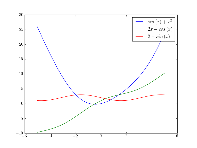
pl.plot(xvals, yvals, label=r"$%s$" % sp.latex(expr))
pl.plot(xvals, dyvals, label=r"$%s$" % sp.latex(dexpr))
pl.plot(xvals, ddyvals, label=r"$%s$" % sp.latex(ddexpr))
pl.legend()
pl.savefig("symbolics_demo.png")

And this is how the output looks like

For many other simple examples, please look at the introductory level sympy tutorial [2].

Note that you should use the computationaly expensive symbolical calculations only in the preparation phase of a numerical simulation program and never in a main computation loop.

Footnotes

[1]	See fore example SyFi which is part of the FEniCS project http://www.fenicsproject.org/

[2]	http://docs.sympy.org/latest/tutorial/index.html