Mayavi2 tips

The mayavi.mlab module, that we call mlab, provides an easy way to visualize data in a script or from an interactive prompt with one-liners as done in the matplotlib pyplot interface but with an emphasis on 3D visualization using Mayavi2. This allows users to perform quick 3D visualization while being able to use Mayavi’s powerful features. For more details see:

• Scripting with mayavi2
• Reference manual

Try:

In [1]: import numpy as np

In [2]: from mayavi import mlab

In [3]: t = np.linspace(0, 2*np.pi, 50)

In [4]: u = np.cos(t)*np.pi

In [5]: x, y, z = np.sin(u), np.cos(u), np.sin(t)

In [6]: mlab.points3d(x,y,z)

In [7]: mlab.show()

In [8]: mlab.points3d(x,y,z,t, scale_mode='none')

In [9]: mlab.show()

In [10]: mlab.points3d?

In [11]: x, y = np.mgrid[-3:3:100j, -3:3:100j ]

In [12]: z = np.sin(x*x + y*y)

In [13]: mlab.surf(x,y,z)

In [14]: mlab.show()

In [15]: mlab.mesh(x,y,z)

In [16]: mlab.show()

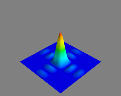
A simple example showing a 3D plot done with the help of mayavi2. The following code shows what it takes to produce such an image. The plotting is essentially only two lines of code!

from numpy import mgrid, real, conj, ones, zeros
from numpy.fft.fftpack import fft2
from numpy.fft.helper import fftshift
from mayavi import mlab

# A mesh grid
X,Y = mgrid[-100:100, -100:100]

# The initial function: a 2D unit step
Z = zeros((200,200))
Z[0:6,0:6] = 0.3*ones((6,6))

# The fourier transform: a 2D sinc(x,y)
W = fftshift(fft2(Z))
W = real(conj(W)*W)

# Display the data with mayavi
# Plot the original function
#mlab.mesh(X, Y, Z)
# Plot the fourier transformed function
mlab.mesh(X, Y, W)
mlab.savefig("mayavi_fft_plot.png")

And now an animated example:

from mayavi import mlab
from scipy import sin, ogrid, array
from pylab import plot, show 

# prepare data, hence test scipy elements
x , y = ogrid[-3:3:100j , -3:3:100j]
z = sin(x**2 + y**2)

# test matplotlib
plot(x, sin(x**2)); show()

#now mayavi2
obj = mlab.surf(x,y,z)
P = mlab.pipeline
scalar_cut_plane = P.scalar_cut_plane(obj, plane_orientation='y_axes')
scalar_cut_plane.enable_contours = True
scalar_cut_plane.contour.filled_contours = True
scalar_cut_plane.implicit_plane.widget.origin = array([  0.00000000e+00,   1.46059210e+00,  -2.02655792e-06])

scalar_cut_plane.warp_scalar.filter.normal = array([ 0.,  1.,  0.])
scalar_cut_plane.implicit_plane.widget.normal = array([ 0.,  1.,  0.])
f = mlab.gcf()
f.scene.camera.azimuth(10)

f.scene.show_axes = True
f.scene.magnification = 4 # or 4
mlab.axes()

# Now animate the data.
dt = 0.01; N = 40
ms = obj.mlab_source
for k in xrange(N):
    x = x + k*dt
    scalars = sin(x**2 + y**2)
    ms.set(x=x, scalars=scalars)

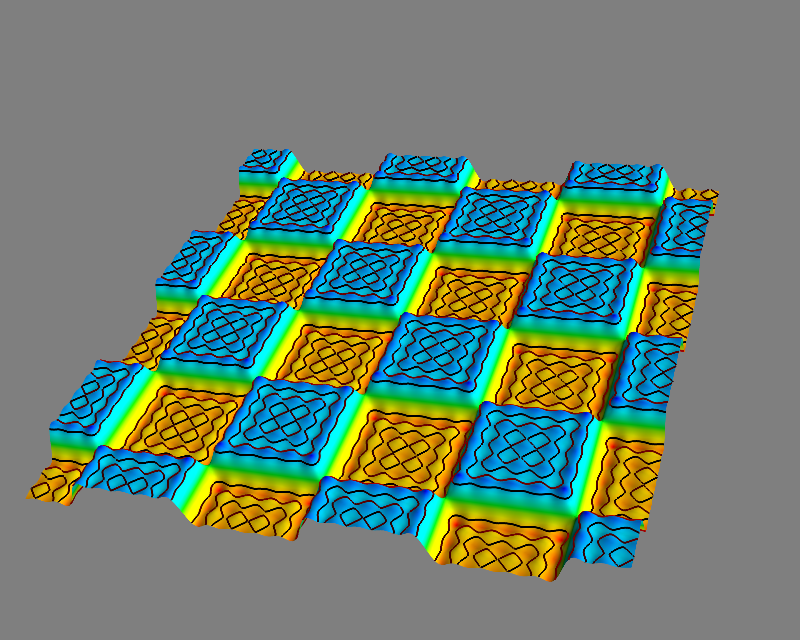
The next example demonstrates how to use scalar cut planes in order to evidence subtle characteristics of a plot. Here, we would like to show the Gibbs oscillations in the Fourier series approximation of jumps.

The workflow for such a problem is:

• write a simple program (let us call it pl.py) that plots your object
• run mayavi2 -x pl.py (python pl.py works too for just executing the script)
• use the ‘spion’ of mayavi2: click on the red point in the menu: the protocol of everything you do visually with the mouse is python-scripted in the opened window
• play with the possibilities and variables that mayavi2 offers, till the image that you see satisfies your exigences
• copy from the ‘spion’-window the relevant information for your result into your pl.py file
• save the picture, if you wish; CAUTION: the pictures that mayavi2 produces became huge, if saved in vector graphics ... so eps is not recommeded here!
• re-run mayavi2 -x pl.py to see if this is really what you wanted
• iterate the above process, if wished
• improve speed and quality of the plot by avoiding rendering and increasing size

In the following code (that was developped following this receipt) you find hints for your formulations.

from numpy import mgrid, zeros, sin, pi, array
from mayavi import mlab

Lx = 4
Ly = 4

S = 10
dx = 0.05
dy = 0.05

# A mesh grid
X,Y = mgrid[-S:S:dx, -S:S:dy]

# The initial function:
#Z = zeros(X.shape)
#Z = sin(pi*X/Lx)*sin(pi*Y/Ly)
#Z[Z>0] = 1
#Z[Z<0] = -1

# The Fourier series:
W = zeros(X.shape)
m = 10
for i in xrange(1,m,2):
    for j in xrange(1,m,2):
        W += 1.0 / (i*j) * sin(i * pi * X / Lx) * sin(j * pi * Y / Ly)
W *= pi / 4.0


# prepare scene
scene = mlab.gcf()
# next two lines came at the very end of the design
scene.scene.magnification = 4

# plot the object
obj = mlab.mesh(X, Y, W)
P = mlab.pipeline

# first scalar_cut_plane
scalar_cut_plane = P.scalar_cut_plane(obj, plane_orientation='z_axes')
scalar_cut_plane.enable_contours = True
scalar_cut_plane.contour.filled_contours = True
scalar_cut_plane.implicit_plane.widget.origin = array([-0.025, -0.025,  0.48])
scalar_cut_plane.warp_scalar.filter.normal = array([ 0.,  0.,  1.])
scalar_cut_plane.implicit_plane.widget.normal = array([ 0.,  0.,  1.])
scalar_cut_plane.implicit_plane.widget.enabled = False # do not show the widget

# second scalar_cut-plane
scalar_cut_plane_2 = P.scalar_cut_plane(obj, plane_orientation='z_axes')
scalar_cut_plane_2.enable_contours = True
scalar_cut_plane_2.contour.filled_contours = True
scalar_cut_plane_2.implicit_plane.widget.origin = array([-0.025, -0.025,  -0.48])
scalar_cut_plane_2.warp_scalar.filter.normal = array([ 0.,  0.,  1.])
scalar_cut_plane_2.implicit_plane.widget.normal = array([ 0.,  0.,  1.])
scalar_cut_plane_2.implicit_plane.widget.enabled = False # do not show the widget

# see it from a closer view point
scene.scene.camera.position = [-31.339891336951567, 14.405281950904936, -27.156389988308661]
scene.scene.camera.focal_point = [-0.025000095367431641, -0.025000095367431641, 0.0]
scene.scene.camera.view_angle = 30.0
scene.scene.camera.view_up = [0.63072643330371414, -0.083217283169475589, -0.77153033000256477]
scene.scene.camera.clipping_range = [4.7116394000124906, 93.313165745624019]
scene.scene.camera.compute_view_plane_normal()

scene.scene.render()